Welcome to debyetools’s documentation!
debyetools is a set of tools written in Python
for the calculation of thermodynamic and thermophysical properties. It’s a library in The Python Package Index (PyPI).
The software presented here is based in the Debye approximation of the quasiharmonic approximation (QHA) using the crystal internal energetics parametrized at ground-state, (go to input file formats to see how DFT calculations results can be used as inputs) to project the thermodynamics properties at high temperatures.
We present here how each contribution to the free energy are considered and a description of the architecture of the calculation engine and of the GUI.
The code is freely available under the GNU Affero General Public License.
How to cite:
If you use debyetools in a publication, please refer to the source code. If you use the implemented method for the calculation of the thermodynamic properties, please cite the following publication:
Jofre, J., Gheribi, A. E., & Harvey, J.-P. Development of a flexible quasi-harmonic-based approach for fast generation of self-consistent thermodynamic properties used in computational thermochemistry. Calphad 83 (2023) 102624. doi: 10.1016/j.calphad.2023.102624.
@article{,
   author = {Javier Jofré and Aïmen E. Gheribi and Jean-Philippe Harvey},
   doi = {10.1016/j.calphad.2023.102624},
   issn = {03645916},
   journal = {Calphad},
   month = {12},
   pages = {102624},
   title = {Development of a flexible quasi-harmonic-based approach for fast generation of self-consistent thermodynamic properties used in computational thermochemistry},
   volume = {83},
   year = {2023},
}
Calculate quality thermodynamic properties in a flexible and fast manner:
It’s possible to couple the Debye model to other algorithms, to fit experimental data and in this way use data available to calculate other properties like thermal expansion, free energy, bulk modulus among many others.

debyetools coupled to a Genetic Algorithm.

Heat capacity of LiFePO4 calculated with debyetools and compared to other methods.
The prediciton of thermodynamic phase equilibria at high pressure can be performed by simultaneous parameter adjusting to experimental heat capacity and thermal expansion at P = 0.

Phase diagram P versus T for the α, β and γ forms of Mg2SiO4. Symbols are literature data for the phase stability regions boundaries.
Using debyetools through the GUI:
debyetools is a Python library that also comes with a graphical user interface to help perform quick calculations without the need to code scripts.
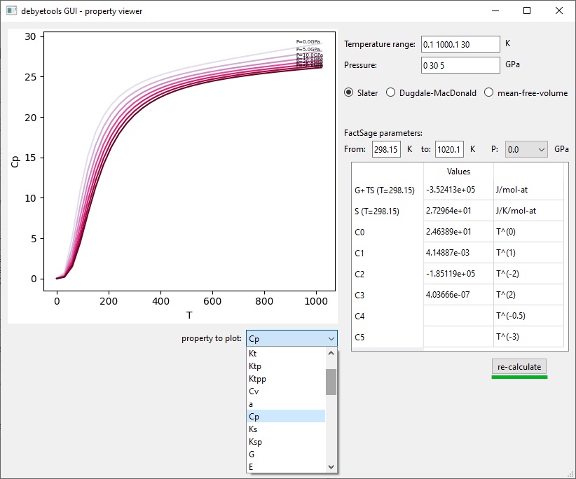
debyetools property viewer.
Using debyetools as a Python library. Example: Al fcc using Morse Potential:
Using debyetools as a Python library adds versatility and expands its usability.
EOS parametrization:
>>> import debyetools.potentials as potentials
>>> from debyetools.aux_functions import load_V_E
>>> V_data, E_data = load_V_E('/path/to/SUMMARY', '/path/to/CONTCAR')
>>> params_initial_guess = [-3e5, 1e-5, 7e10, 4]
>>> formula = 'AlAlAlLi'
>>> cell = np.array([[4.025,0,0],[0,4.025488,0],[0,0,4.025488]])
>>> basis = np.array([[0,0,0],[.5,.5,0],[.5,0,.5],[0,.5,.5]])
>>> cutoff, number_of_neighbor_levels = 5, 3
>>> Morse = potentials.MP(formula, cell, basis, cutoff,
...                       number_of_neighbor_levels)
>>> Morse.fitEOS(V_data, E_data, params_initial_guess)
array([-3.26551e+05,9.82096e-06,6.31727e+10,4.31057e+00])
Calculation of the electronic contribution:
>>> from debyetools.aux_functions import load_doscar
>>> from debyetools.electronic import fit_electronic
>>> p_el_inittial = [3.8e-01,-1.9e-02,5.3e-04,-7.0e-06]
>>> E, N, Ef = load_doscar('/path/to/DOSCAR.EvV.',list_filetags=range(21))
>>> fit_electronic(V_data, p_el_inittial, E, N, Ef)
array([1.73273079e-01,-6.87351153e+03,5.3e-04,-7.0e-06])
Poisson’s ratio:
>>> import numpy as np
>>> from debyetools . poisson import poisson_ratio
>>> from debyetools.aux_functions import load_EM
>>> EM = load_EM( 'path/to/OUTCAR')
>>> poisson_ratio ( EM )
0.2 2 9 41 5 49 8 67148558
Free energy minimization:
>>> from debyetools.ndeb import nDeb
>>> from debyetools import potentials
>>> from debyetools.aux_functions import gen_Ts,load_V_E
>>> m = 0.021971375
>>> nu = poisson_ratio (EM)
>>> p_electronic = fit_electronic(V_data, p_el_inittial, E, N, Ef)
>>> p_defects = [8.46, 1.69, 933, 0.1]
>>> p_anh, p_intanh = [0,0,0], [0, 1]
>>> V_data, E_data = load_V_E('/path/to/SUMMARY', '/path/to/CONTCAR')
>>> eos = potentials.BM()
>>> peos = eos.fitEOS(V_data, E_data, params_initial_guess)
>>> ndeb = nDeb (nu , m, p_intanh , eos , p_electronic , p_defects , p_anh )
>>> T = gen_Ts ( T_initial , T_final , 10 )
>>> T, V = ndeb.min_G (T,  1e-5, P=0)
>>> V
array([9.98852539e-06, 9.99974297e-06, 1.00578469e-05, 1.01135875e-05,
       1.01419825e-05, 1.02392921e-05, 1.03467847e-05, 1.04650048e-05,
       1.05953063e-05, 1.07396467e-05, 1.09045695e-05, 1.10973163e-05])
Evaluation of the thermodynamic properties:
>>> trprops_dict=ndeb.eval_props(T,V)
>>> tprops_dict['Cp']
array([4.02097531e-05, 9.68739597e+00, 1.96115210e+01, 2.25070513e+01,
       2.34086394e+01, 2.54037595e+01, 2.68478029e+01, 2.82106379e+01,
       2.98214145e+01, 3.20143195e+01, 3.51848547e+01, 3.98791392e+01])
FS compound database parameters:
>>> from debyetools.fs_compound_db import fit_FS
>>> T_from = 298.15
>>> T_to = 1000.1
>>> FS_db_params = fit_FS(tprops_dict, T_from,T_to)
>>> Fs_db_params['Cp']
array([ 3.48569519e+01, -2.56558596e-02, -6.35562885e+05,  2.65035585e-05])