Examples
Table of contents
Al3Li L12 thermodynamic properties
In order to calculate the thermodynamic properties of an element or compound, we need first to parametrize the function that will describe the internal energy of the system.
In this case we have chosen the Birch-Murnaghan equation of state and fitted it against DFT data loaded using the load_V_E function.
The BM object instantiates the representation og the EOS and its derivatives. In the module potentials there are all the implemented EOS.
The method fitEOS with the option fit=True will fit the EOS parameters to (Volume, Energy) data using initial_parameters as initial guess.
The following is an example for Al3Li L12.
The following code allows to access the example files:
>>> import os
>>> import debyetools
>>> file_path = debyetools.__file__
>>> dir_path = os.path.dirname(file_path)
Loading the energy curve and fitting the Birch-Murnaghan EOS:
>>> from debyetools.aux_functions import load_V_E
>>> import debyetools.potentials as potentials
>>> import numpy as np
>>> V_DFT, E_DFT = load_V_E(dir_path+'/examples/Al3Li_L12/SUMMARY.fcc', dir_path+'/examples/Al3Li_L12/CONTCAR.5', units='J/mol')
>>> initial_parameters =  np.array([-4e+05, 1e-05, 7e+10, 4])
>>> eos_BM = potentials.BM()
>>> eos_BM.fitEOS(V_DFT, E_DFT, initial_parameters=initial_parameters, fit=True)
>>> p_EOS = eos_BM.pEOS
>>> p_EOS
array([-3.26544606e+05,  9.82088168e-06,  6.31181335e+10,  4.32032416e+00])
To fit the electronic contribution to eDOS data we can load them as VASP format DOSCAR files using the function load_doscar.
Then, at each V_DFT volume, the parameters of the electronic contribution will be fitted with the fit_electronic function from the electronic module, using p_el_initial as initial parameters.
>>> from debyetools.aux_functions import load_doscar
>>> from debyetools.electronic import fit_electronic
>>> p_el_inittial = [3.8027342892e-01, -1.8875015171e-02, 5.3071034596e-04, -7.0100707467e-06]
>>> E, N, Ef = load_doscar(dir_path+'/examples/Al3Li_L12/DOSCAR.EvV.')
>>> p_electronic = fit_electronic(V_DFT, p_el_inittial,E,N,Ef)
>>> p_electronic
array([ 1.73372534e-01, -6.87754210e+03,  5.30710346e-04, -7.01007075e-06])
The Poisson’s ratio and elastic constants can be calculated using the poisson_ratio method and the elastic moduli matrix in the VASP format OUTCAR obtained when using IBRION = 6 in the INCAR file, loaded using load_EM.
>>> from debyetools.aux_functions import load_EM
>>> from debyetools.poisson import poisson_ratio
>>> EM = load_EM(dir_path+'/examples/Al_fcc/OUTCAR.eps')
>>> nu = poisson_ratio(EM)
>>> nu
0.33702122500881493
For this example, all other contributions are set to zero.
>>> Tmelting = 933
>>> p_defects = 1e10, 0, Tmelting, 0.1
>>> p_intanh = 0, 1
>>> p_anh = 0, 0, 0
The temperature dependence of the equilibrium volume is calculated by minimizing G. In this example is done at P=0. We need to instantiate first a nDeb object and define the arbitrary temperatures (this can be done using gen_Ts, for example).
The minimization og the Gibbs free energy is done by calling the method nDeb.minG.
>>> from debyetools.ndeb import nDeb
>>> from debyetools.aux_functions import gen_Ts
>>> m = 0.026981500000000002
>>> ndeb_BM = nDeb(nu, m, p_intanh, eos_BM, p_electronic, p_defects, p_anh)
>>> T_initial, T_final, number_Temps = 0.1, 1000, 10
>>> T = gen_Ts(T_initial, T_final, number_Temps)
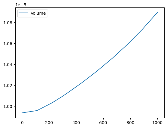
>>> T, V = ndeb_BM.min_G(T,p_EOS[1],P=0)
>>> T, V
(array([1.0000e-01, 1.1120e+02, 2.2230e+02, 2.9815e+02, 3.3340e+02,
4.4450e+02, 5.5560e+02, 6.6670e+02, 7.7780e+02, 8.8890e+02,
1.0000e+03]),
array([9.93477130e-06, 9.95708573e-06, 1.00309860e-05, 1.00924551e-05,
1.01230085e-05, 1.02253260e-05, 1.03361669e-05, 1.04567892e-05,
1.05882649e-05, 1.07335434e-05, 1.08954899e-05]))
To plot the volume as function of temperature:
>>> from matplotlib import pyplot as plt
>>> plt.figure()
>>> plt.plot(T,V, label='Volume')
>>> plt.legend()
>>> plt.show()
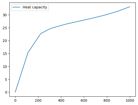
The thermodynamic properties are calculated by just evaluating the thermodynamic functions with nDeb.eval_props. This will return a dictionary with the values of the different thermodynamic properties.
>>> tprops_dict = ndeb_BM.eval_props(T,V,P=0)
>>> Cp = tprops_dict['Cp']
>>> Cp
array([4.03108486e-05, 1.53280407e+01, 2.26806532e+01, 2.44706878e+01,
       2.50389680e+01, 2.63913291e+01, 2.75000371e+01, 2.86033148e+01,
       2.98237204e+01, 3.12758030e+01, 3.31133279e+01])
>>> plt.figure()
>>> plt.plot(T,Cp, label='Heat capacity')
>>> plt.legend()
>>> plt.show()
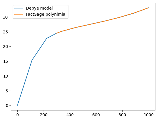
The FactSage Cp polynomial is fitted to the previous calculation:
>>> from debyetools.fs_compound_db import fit_FS
>>> T_from = 298.15
>>> T_to = 1000
>>> FS_db_params = fit_FS(tprops_dict, T_from, T_to)
>>> FS_db_params
{'Cp': array([ 2.82760954e+01, -6.12271903e-03, -2.66975291e+05,  1.11891931e-05]),
 'a': array([-8.00942545e-05,  1.65169216e-07,  6.62935957e-02, -9.59227812e+00]),
 '1/Ks': array([ 1.58260299e-11,  3.89418226e-15, -1.26886122e-18,  2.36654487e-21]),
 'Ksp': array([4.50472269e+00, 1.16376200e-03])}
Plot the parameterized heat capacity:
Thermodynamic properties with the debyetools interface
The same calculations as the previous example were carried out using debyetools GUI.
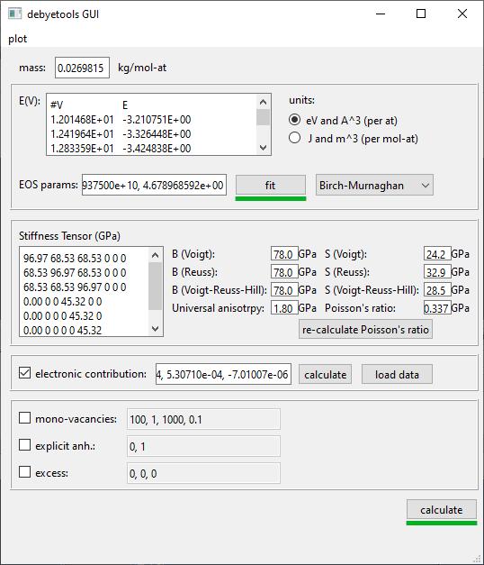
debyetools main interface
The calculated results can be plotted in the viewer window that will pop-up after clicking the button ‘calculate’. Note that the number of calculations where modified from default settings to show smoother curves.
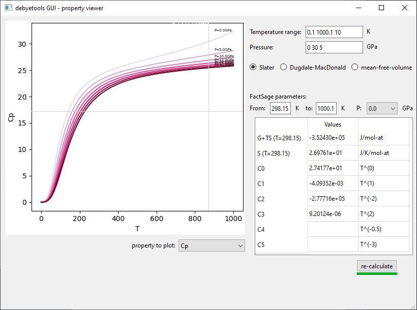
debyetools viewer window
Genetic algorithm to fit Cp to experimental data.
To show how flexible debyetools is we shoe next a way to fit a thermodynamic property like the heat capacity to experimental data using a genetic algorithm.

Schematics for data fitting o the heat capacity to experimental data.
First we set the initial input values and experimental values:
>>> import numpy as np
>>> import debyetools.potentials as potentials
>>> eos_MU = potentials.MU()
>>> params_Murnaghan = [-6.745375544e+05, 6.405559904e-06, 1.555283892e+11, 4.095209375e+00]
>>> E0, V0, K0, K0p = params_Murnaghan
>>> nu = 0.2747222272342077
>>> a0, m0 = 0, 1
>>> s0, s1, s2 = 0, 0, 0
>>> edef, sdef = 20,0
>>> T = np.array([126.9565217,147.826087,167.826087,186.9565217,207.826087,226.9565217,248.6956522,267.826087,288.6956522,306.9565217,326.9565217,349.5652174,366.9565217,391.3043478,408.6956522,428.6956522,449.5652174,467.826087,488.6956522,510.4347826,530.4347826,548.6956522,571.3043478,590.4347826,608.6956522,633.0434783,649.5652174,670.4347826,689.5652174,711.3043478,730.4347826,750.4347826,772.173913])
>>> C_exp = np.array([9.049180328,10.14519906,11.29742389,12.05620609,12.92740047,13.82669789,14.61358314,15.45667447,16.07494145,16.55269321,17.00234192,17.73302108,18.21077283,18.60421546,19.25058548,19.53161593,19.78454333,20.12177986,20.4028103,20.90866511,21.18969555,21.52693208,21.89227166,22.4824356,22.96018735,23.40983607,23.69086651,23.88758782,23.71896956,23.7470726,23.85948478,23.83138173,24.19672131])
Then we run a genetic algorithm to fit the heat capacity to the experimental data.
>>> import numpy.random as rnd
>>> from debyetools.ndeb import nDeb
>>> ix = 0
>>> max_iter = 500
>>> mvar=[(V0,V0*0.01), (K0,K0*0.05), (K0p,K0p*0.01), (nu,nu*0.01), (a0,5e-6), (m0,5e-3), (s0,5e-5), (s1,5e-5), (s2,5e-5), (edef,0.5), (sdef, 0.1)]
>>> parents_params = mutate(params = [V0, K0, K0p, nu, a0, m0, s0, s1, s2, edef, sdef], n_chidren = 2, mrate=0.7, mvar=mvar)
>>> counter_change = 0
>>> errs_old = 1
>>> while ix <= max_iter:
...    children_params = mate(parents_params, 10, mvar)
...    parents_params, errs_new = select_bests(Cp_LiFePO4, T, children_params,2, C_exp)
...    V0, K0, K0p, nu, a0, m0, s0, s1, s2, edef, sdef = parents_params[0]
...    mvar=[(V0,V0*0.05), (K0,K0*0.05), (K0p,K0p*0.05), (nu,nu*0.05), (a0,5e-6), (m0,5e-3), (s0,5e-5), (s1,5e-5), (s2,5e-5), (edef,0.5), (sdef, 0.1)]
...    if errs_old == errs_new[0]:
...        counter_change+=1
...    else:
...        counter_change=0
...    ix+=1
...    errs_old = errs_new[0]
...    if counter_change>=20: break
>>> T = np.arange(0.1,800.1,20)
>>> Cp1 = Cp_LiFePO4(T, parents_params[0])
>>> best_params = parents_params[0]
The algorithm consists in first generating the parent set of parameters by running mutate function with the option n_children = 2 to generate two variation of the initial set.
Then the iterations goes by (1) mating the parents using the function mate, (2) evaluating and (3) selecting the best 2 sets that will be the new parents. This will go until stop conditions are met.
The mate, mutate, select_bests and evaluate are as follows:
def mutate(params, n_chidren, mrate, mvar):
    res = []
    for i in range(n_chidren):
        new_params = []
        for pi, mvars in zip(params, mvar):
            if rnd.randint(0,100)/100.<=mrate:
                step = mvars[1]/10
                lst1 = np.arange(mvars[0]-mvars[1], mvars[0]+mvars[1]+step, step )
                var = lst1[rnd.randint(0,len(lst1))]
                new_params.append(var)
            else:
                new_params.append(pi)

        res.append(new_params)
    return res

def evaluate(fc, T, pi, yexp):
    return np.sqrt(np.sum((fc(T, pi)/T - yexp/T)**2))
    try:
        return np.sqrt(np.sum((fc(T, pi)/T - yexp/T)**2))
    except:
        print('these parameters are not working:',pi)
        return 1

def select_bests(fn, T, params, ngen, yexp):
    arr = []
    for ix, pi in enumerate(params):
        arr.append([ix, evaluate(fn, T, pi, yexp)])

    arr = np.array(arr)
    sorted_arr = arr[np.argsort(arr[:, 1])]
    tops_ix = sorted_arr[:ngen,0]

    return [params[int(j)] for j in tops_ix], [arr[int(j),1] for j in tops_ix]

def mate(params, ngen,mvar):
    res = [params[0],params[1]]
    ns = int(max(2,ngen-2)/2)

    for i in range(ns):
        cutsite = rnd.randint(0,len(params[0]))
        param1 = mutate(params[0][:cutsite]+params[1][cutsite:], 1, 0.5, mvar)[0]
        param2 = mutate(params[1][:cutsite]+params[0][cutsite:], 1, 0.5, mvar)[0]

        res.append(param1)
        res.append(param2)

    return res
The function to evaluate, the heat capacity, is as follows:
def Cp_LiFePO4(T, params):
    V0, K0, K0p, nu, a0, m0, s0, s1, s2, edef, sdef = params
    p_intanh = a0, m0
    p_anh = s0, s1, s2

    # EOS parametrization
    #=========================
    initial_parameters =  [-6.745375544e+05, V0, K0, K0p]
    eos_MU.fitEOS([V0], 0, initial_parameters=initial_parameters, fit=False)
    p_EOS = eos_MU.pEOS
    #=========================

    # Electronic Contributions
    #=========================
    p_electronic = [0,0,0,0]
    #=========================

    # Other Contributions parametrization
    #=========================
    Tmelting = 800
    p_defects = edef, sdef, Tmelting, 0.1
    #=========================

    # F minimization
    #=========================
    m = 0.02253677142857143
    ndeb_MU = nDeb(nu, m, p_intanh, eos_MU, p_electronic,
                    p_defects, p_anh, mode='jj)
    T, V = ndeb_MU.min_G(T, p_EOS[1], P=0)
    #=========================

    # Evaluations
    #=========================
    tprops_dict = ndeb_MU.eval_props(T, V, P=0)
    #=========================

    return tprops_dict['Cp']
The result of this fitting can be plotted using the plotter module:
import debyetools.tpropsgui.plotter as plot

T_exp = np.array([126.9565217,147.826087,167.826087,186.9565217,207.826087,226.9565217,248.6956522,267.826087,288.6956522,306.9565217,326.9565217,349.5652174,366.9565217,391.3043478,408.6956522,428.6956522,449.5652174,467.826087,488.6956522,510.4347826,530.4347826,548.6956522,571.3043478,590.4347826,608.6956522,633.0434783,649.5652174,670.4347826,689.5652174,711.3043478,730.4347826,750.4347826,772.173913])
Cp_exp = np.array([9.049180328,10.14519906,11.29742389,12.05620609,12.92740047,13.82669789,14.61358314,15.45667447,16.07494145,16.55269321,17.00234192,17.73302108,18.21077283,18.60421546,19.25058548,19.53161593,19.78454333,20.12177986,20.4028103,20.90866511,21.18969555,21.52693208,21.89227166,22.4824356,22.96018735,23.40983607,23.69086651,23.88758782,23.71896956,23.7470726,23.85948478,23.83138173,24.19672131])
T_ph = [1.967263911, 24.08773869, 40.16838464, 51.99817063, 62.61346532, 71.62728127, 82.14182721, 95.16347545, 108.6874128, 123.7174904, 140.2528445, 158.7958422, 179.3467704, 202.4077519, 226.4743683, 250.5441451, 274.6162229, 299.1922033, 323.2681948, 347.8476048, 371.9269543, 396.0073777, 420.0891204, 444.171937, 468.7572464, 492.8416261, 516.9264916, 541.5140562, 565.6001558, 589.6869304, 613.7740731, 638.3634207, 662.4510066, 686.0373117, 711.1294163, 734.2134743, 764.3270346]
Cp_ph =[-0.375850956, -0.178378686, 1.227397939, 2.313383473, 3.431619848, 4.344789455, 5.478898585, 6.723965937, 7.953256737, 9.166990283, 10.40292814, 11.64187702, 12.87129914, 14.08268875, 15.21632722, 16.2118242, 17.10673273, 17.9153379, 18.63917154, 19.29786266, 19.87491167, 20.4050194, 20.87745642, 21.30295216, 21.70376428, 22.06093438, 22.39686914, 22.69910457, 22.98109412, 23.23357771, 23.46996716, 23.69426517, 23.91128202, 24.1000059, 24.28807125, 24.49073617, 24.58375529]

T_JJ = [1.00000E-01,1.64245E+01,3.27490E+01,4.90735E+01,6.53980E+01,8.17224E+01,9.80469E+01,1.14371E+02,1.30696E+02,1.47020E+02,1.63345E+02,1.79669E+02,1.95994E+02,2.12318E+02,2.28643E+02,2.44967E+02,2.61292E+02,2.77616E+02,2.93941E+02,2.98150E+02,3.10265E+02,3.26590E+02,3.42914E+02,3.59239E+02,3.75563E+02,3.91888E+02,4.08212E+02,4.24537E+02,4.40861E+02,4.57186E+02,4.73510E+02,4.89835E+02,5.06159E+02,5.22484E+02,5.38808E+02,5.55133E+02,5.71457E+02,5.87782E+02,6.04106E+02,6.20431E+02,6.36755E+02,6.53080E+02,6.69404E+02,6.85729E+02,7.02053E+02,7.18378E+02,7.34702E+02,7.51027E+02,7.67351E+02,7.83676E+02,8.00000E+02]
Cp_JJ = [Cp_LiFePO4(T, params_Murnaghan) for T in T_JJ]
Cp_JJ_fitted = [Cp_LiFePO4(T, best_params) for T in T_JJ]

fig = plot.fig(r'Temperature$~\left[K\right]$', r'$C_P~\left[J/K-mol-at\right]$')

fig.add_set(T_exp, Cp_exp, label = 'exp', type='dots')
fig.add_set(T_ph, Cp_ph, label = 'phonon', type='dash')
fig.add_set(T_JJ, Cp_JJ, label = 'Murnaghan', type='line')
fig.add_set(T_JJ_fit, Cp_JJ_fit, label = 'Murnaghan+fitted', type='line')
fig.plot(show=True)
The resulting figure is:

LiFePO4 heat capacity.
Simultaneous parameter adjusting to experimental heat capacity and thermal expansion at P = 0 and prediction of thermodynamic phase equilibria at high pressure
Similarly to the previous example, a genetic algorithm was implemented to adjust model parameters fitting experimental data. The compound studied was Mg$_2$SiO$_4$ in the $alpha$, $beta$, and $gamma$ phases (forsterite, wadsleyite, and ringwoodite) with structures Pnma, Imma, and Fd3m, respectively, for temperatures from $0$ to $2500~K$ and pressures from $0$ to $30~GPa$. In this usage example, the isobaric heat capacity and the thermal expansion were fitted simultaneously at $0$ pressure. For that, the objective function should simultaneously evaluate the thermal expansion and heat capacity as:
def Cp_alpha_Mg2SiO4(T, params):
    V0, K0, K0p, nu, a0, m0, s0, s1, s2, edef, sdef = params
    p_intanh = a0, m0
    p_anh = s0, s1, s2
    initial_parameters =  [-6.745375544e+05, V0, K0, K0p]
    eos_MU.fitEOS([V0], 0, initial_parameters=initial_parameters, fit=False)
    p_EOS = eos_MU.pEOS
    p_electronic = [0,0,0,0]
    Tmelting = 800
    p_defects = edef, sdef, Tmelting, 0.1
    m = 0.02253677142857143
    ndeb_MU = nDeb(nu, m, p_intanh, eos_MU, p_electronic,
                    p_defects, p_anh, mode='jj)
    T, V = ndeb_MU.min_G(T, p_EOS[1], P=0)
    tprops_dict = ndeb_MU.eval_props(T, V, P=0)
    return [tprops_dict['a'], tprops_dict['Cp']]
The genetic algorithms remains the same as the previous example except for the evaluation function which now takes target data for both thermal expansion and heat capacity.
def evaluate(fc, T_set1, T_set2, pi, yexp, yexp2):
    evalfunc1 = fc(T_set1, pi, eval='min')
    evalfunc2 = fc(T_set2, pi, eval='min')
    try:
        errtotal1 = np.sqrt(np.sum(((evalfunc1[0] - yexp) / yexp) ** 2)) / len(T_set1)
        errtotal2 = np.sqrt(np.sum(((evalfunc2[1] - yexp2) / yexp2) ** 2)) / len(T_set2)
        return errtotal1 + errtotal2
    except:
        return 1e10
Once the optimal parameters for the three phases are obtained, the calculation of the thermodynamic properties can be calculated as function of the temperature and pressure as:
Ps = gen_Ps(0, 30e9, n_vals)

tprops_dict = []

# Pressure loop:
for P in Ps:
    # minimization of the free energy:
    T, V = ndeb.min_G(Ts, V0, P=P)
    # evaluation of the thermodynamic properties:
    tprops_dict.append(ndeb.eval_props(T, V, P=P))
In order to access the Gibbs free energy of each phase we use the key G in the tprops_dict list. Note that this list stores, for each pressure, a dictionary with all the thermodynamic properties.
G_alpha = np.zeros((len(Ts), len(Ps)))
G_beta = np.zeros((len(Ts), len(Ps)))
G_gamma = np.zeros((len(Ts), len(Ps)))
for i in range(len(Ts)):
    for j in range(len(Ps)):
        G_alpha[i, j] = tprops_dict_alpha[j]['G'][i]
        G_beta[i, j] = tprops_dict_beta[j]['G'][i]
        G_gamma[i, j] = tprops_dict_gamma[j]['G'][i]
To evaluate the stability relative to these three phases, the Gibbs free energy of each of them is compared:
G_z = np.zeros((len(Ts), len(Ps)))
for i in range(len(Ts)):
    for j in range(len(Ps)):
        G_list = [tprops_dict_alpha[j]['G'][i], tprops_dict_beta[j]['G'][i], tprops_dict_gamma[j]['G'][i]]
        print(G_list)
        G_z[j,i] = G_list.index(min(G_list)) +1
This can be plotted in a P vs T predominance diagram:

Phase diagram P versus T for the α, β and γ forms of Mg2SiO4. Symbols are literature data for the phase stability regions boundaries.